

What actually breaks first in production
Imagine the run after the obvious transport fixes. DBO is enabled, the DeepEP mode looks reasonable, the fabric is no longer the only visible bottleneck, and throughput still flattens. At that point the question changes from "what is the communication model?" to "what is stretching the step in production?"
Parts 1 and 2 gave us the operating model: keep per-rank work large enough to cover communication, choose the DeepEP kernel family by measured payload regime, and watch for the topology boundary where the fast fabric gives way to scale-out networking.
The remaining failures are rarely exotic. Most bad Wide-EP traces reduce to one of five patterns:
- the per-rank work is too small, so DBO has nothing to hide,
- the critical fabric is saturated or jittery,
- communication buffers are fighting with KV cache for HBM,
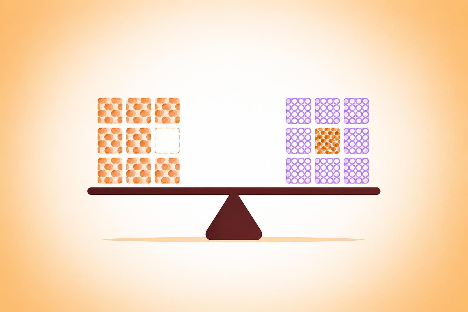
- a few hot experts create slow ranks and stretch the whole step,
- the software stack assumes a transport model that does not match the hardware you actually have.
This final part focuses on the last two. They are where "the math was fine" often turns into "the deployment still did not scale."
The reason this matters commercially is straightforward: production inference failures do not usually announce themselves as clean model errors. They show up as extra machines with poor utilization, fragile throughput under bursty traffic, and unclear ownership between model, kernel, network, and scheduler teams. A good serving stack needs a way to tell those failure modes apart quickly.
1) Failure modes to recognize quickly
Name the failure mode before touching another knob:
- DBO did not help. The per-rank compute slice is probably too small. The first fix to try is a larger effective \(B\), not endless overlap tuning.
- The slow fabric is noisy. Lower average \(BW_{\text{eff}}\) hurts, but variance is worse: jitter breaks the assumption that communication can stay hidden under compute.
- Memory pressure is eating the margin. Double buffers, DeepEP buffers, redundant experts, and KV cache all compete for the same HBM headroom.
- A few ranks are hot. When one or two GPUs consistently receive more routed work, the whole EP group waits for them.
- The topology assumption is wrong. The algorithm may be fine, but the chosen communication path assumes a transport property the actual platform does not provide cheaply.
The trap is treating every bad trace as a transport trace. Once a few ranks are systematically slower, changing the kernel backend can improve the margins while leaving the real bottleneck untouched.
A quick diagnosis map
Symptom in the traceLikely failure modeMetric to check firstFirst actionDBO is enabled but throughput barely movesNot enough compute coverPer-rank tokens, expert kernel time, DBO fill/drain overheadIncrease effective batch or raise DBO thresholdsAverage bandwidth looks acceptable but tail latency spikesFabric jitterPer-collective latency distribution, not just mean \(BW_{\text{eff}}\)Separate local and scale-out bytes; remeasure by topologyThroughput drops when overlap/buffers are enabledHBM pressureKV cache headroom, DeepEP buffer size, allocator pressureReduce buffer footprint before adding replicasOne rank repeatedly finishes lateHot experts / load skewPer-rank routed tokens, per-expert token counts, \(\gamma\)Evaluate EPLB before changing transportPerformance changes sharply across hardwareTopology mismatchLocal versus remote traffic split, NIC behavior, ordering/atomic assumptionsRevisit communication path and portability layer
This table is intentionally simple. It is not a replacement for profiling; it is a guardrail against chasing the wrong subsystem for a week.
2) EPLB: spend memory to shrink the slowest rank
The scalar to watch is still
$$\gamma = \frac{\max_r \text{load}_r}{\operatorname{mean}_r \text{load}_r}$$
where "load" is the routed token load on each rank, or a better proxy if you have one.
When a few experts are consistently hot, the ranks hosting them become the stragglers. EPLB attacks that problem by spending memory on redundant expert copies.
The public EPLB README describes the approach as redundant experts:
- identify heavy-loaded experts,
- duplicate them,
- repack the duplicates to reduce the peak load across GPUs.
It also distinguishes two policies:
- hierarchical load balancing, which tries to keep expert groups aligned with nodes when the topology makes that worthwhile,
- global load balancing, which ignores the grouping structure and balances across the whole EP group.
The vLLM defaults are conservative
In current vLLM, EPLBConfig defaults to:
window_size = 1000step_interval = 3000num_redundant_experts = 0use_async = falselog_balancedness = false
That conservative default is right. Do not spend HBM on redundant experts until the trace shows that hot ranks are the problem.
There are a few enablement constraints worth keeping in mind. Current vLLM requires expert parallelism to be enabled, requires the tensor-parallel or data-parallel size to be greater than one, and rejects a nonzero num_redundant_experts unless EPLB itself is enabled. The current implementation also supports CUDA-like platforms, including CUDA and ROCm devices.
Why this helps
Under the reduced model from Parts 1 and 2,
$$t_{\text{compute}} \approx \gamma \cdot \frac{B\,k}{P} \cdot c_{\text{tok}}$$
EPLB therefore acts directly on the multiplicative penalty. If the hottest rank is consistently pulling the step long, lowering \(\gamma\) can matter more than shaving a few more microseconds from the all-to-all.
For example, if \(\gamma = 1.35\), the hottest rank is stretching the expert-compute portion of the step by roughly 35% relative to the balanced case. If expert compute is already the exposed part of the pipeline, reducing \(\gamma\) toward 1.05 can matter more than improving the communication kernel by a small constant factor. The win comes from shortening the rank everyone waits for.
The trade-off is memory. A useful first-order estimate is
$$\text{extra HBM} \approx \frac{R \cdot N_{\text{MoE layers}} \cdot \text{bytes per expert}}{P}$$
where \(R\) is the number of redundant expert copies per MoE layer across the EP group. Calculate that cost from the actual checkpoint and precision format; do not inherit a rule of thumb from somebody else's deployment.
That memory trade-off is why EPLB should be treated as a capacity decision, not just a performance knob. Every redundant expert competes with KV cache, activation buffers, communication buffers, and safety headroom. If the service is already memory-bound, replication can improve balance while making admission control worse.
A practical way to use it
Use EPLB only after the trace points to persistent rank imbalance. A reasonable rollout sequence is:
- confirm that the slowest ranks are also the ranks receiving the hottest expert traffic,
- start with a small
num_redundant_expertsvalue and measure the change in \(\gamma\), - keep
window_sizeandstep_intervalnear their defaults unless the routing distribution changes faster than those windows can track.
If the workload is fairly stationary, aggressive rebalancing can add noise without improving the critical path.
The best sign that EPLB is working is not just a prettier expert histogram. It is a narrower step-time distribution, lower hottest-rank load, and no unacceptable loss of memory headroom. If \(\gamma\) improves but throughput does not, the bottleneck was probably elsewhere.
3) LPLB: the per-batch version of the same idea
LPLB pushes the same load-balancing idea into the current batch. Instead of reacting to a historical window, it solves a minimax linear program over the redundant-expert graph. The README describes the core problem as:
$$\begin{alignedat}{3} \min_{f, z}\quad & z \\ \text{subject to}\quad & \ell_g = w_g - \sum_{e \in \text{out}(g)} f_e + \sum_{e \in \text{in}(g)} f_e && \forall\, g \\ & \ell_g \le z && \forall\, g \\ & 0 \le f_e \le c_e && \forall\, e \in E \end{alignedat}$$
Here \(w_g\) is the initial load on replica group \(g\), \(f_e\) is the flow moved along redundancy edge \(e\), \(c_e\) is that edge's capacity, \(\ell_g\) is the resulting load, and \(z\) is the maximum load being minimized.
The distinction is simple:
- EPLB reacts to historical average load,
- LPLB reacts to the current batch.
That makes LPLB attractive when batch-to-batch variance is large enough that static replication leaves performance on the table.
The current project framing is closer to training and research than to a drop-in inference default. That does not make the idea irrelevant for serving, but it does mean I would treat it as a technique to evaluate, not a production knob to flip casually.
The key difference is time scale. EPLB asks, "which experts have been hot over the recent window?" LPLB asks, "given this batch and this redundancy graph, how should tokens be reassigned right now?" That distinction matters when the routing distribution changes faster than a historical moving average can track.
The practical decision rule is:
- use EPLB when skew is persistent and predictable,
- consider LPLB when skew is bursty enough that windowed statistics lag behind,
- avoid both when the trace is still dominated by transport, memory pressure, or too-small per-rank work.
The caveats matter more than the acronym
The LPLB README is refreshingly explicit about its own limitations:
- the current planner balances token count, not true grouped-GEMM runtime,
- the solver is about 100 microseconds intra-node and longer inter-node,
- the project is still in an early research stage.
So do not treat LPLB as a strict upgrade over EPLB. Treat it as a candidate tool once you have shown that:
- hot-rank behavior is your limiting factor,
- the imbalance is bursty enough that historical windows miss it,
- the LP overhead is worth paying relative to the saved compute time.
For production inference today, EPLB is still the conservative answer. In this part of the stack, conservative is often correct.
If LPLB becomes part of a serving path, I would want to see three things before trusting it: the LP overhead as a fraction of step time, the improvement in tail rank load, and a comparison against a well-tuned EPLB baseline on the same traffic. Without those, it is easy to mistake a more sophisticated optimizer for a better production system.
4) Portability is mostly a control-plane question
DeepEP is fast partly because it is tightly coupled to the NVIDIA stack. That is also why portability is not automatic.
The UCCL-EP preview is interesting because it keeps the expert-parallel communication shape while moving part of the networking control plane back to CPU proxies:
- the GPU still performs the data-intensive work such as packing, forwarding, and overlap-friendly local operations,
- lightweight control commands are forwarded to CPU-side proxies,
- those proxies handle queue management, flow control, and NIC verbs.
That design matters most on fabrics that do not behave like the assumptions baked into NVIDIA-specific paths. AWS EFA / SRD is the obvious example, but heterogeneous GPU/NIC pairings matter too.
This is the portability lesson for serving teams: the hard part is not only rewriting kernels. The hard part is preserving the contract that the runtime expects from the network. Ordering, completion, queue pressure, atomics, and congestion behavior all affect whether dispatch/combine can be overlapped safely. A kernel that is fast on one vendor stack can become fragile when those control-plane assumptions change.
UCCL-EP is interesting because it separates the data path from the control path. The GPU still does the high-throughput local work; the CPU proxy handles the parts that need visibility into the NIC and transport. That is a useful architecture pattern even beyond UCCL itself.
How strongly should you trust the published UCCL-EP numbers?
The UCCL-EP full-results post and paper report several application-level results:
- up to 45% higher Megatron-LM training throughput over RCCL on 128 AMD GPUs in the MI300X + Broadcom setup,
- up to 40% higher SGLang inference throughput over NCCL in the Qwen3 p5en / H200 + EFA setup,
- up to 25% lower vLLM TPOT over NCCL on a two-node H200 + EFA setup.
They also report detailed H200 + EFA dispatch/combine bandwidth measurements, plus broader AMD, Broadcom, and Pollara results. Treat these as project-reported measurements, not industry consensus. The directional claim is useful, but the exact deltas should still be rechecked against the latest UCCL-EP benchmark page before being used in production planning.
The architectural lesson is more durable than the exact deltas:
the algorithmic shape of expert-parallel communication is more portable than the original DeepEP plumbing makes it look.
That is a useful thing to know even if you never deploy UCCL-EP itself.
For a public-cloud buyer, the implication is important: EP performance should not be evaluated only by asking whether a platform has fast GPUs. You also need to ask whether the serving stack can express the right communication pattern on that GPU/NIC pair without relying on assumptions that only hold on a vertically integrated NVIDIA path.
5) The shortest operator checklist
The whole series reduces to a short production checklist:
- Check whether the per-rank work is large enough for DBO to matter at all.
- Verify which fabric is actually on the critical path and remeasure \(BW_{\text{eff}}\) after every topology change.
- Only reach for EPLB or LPLB after you have evidence that hot ranks, not transport, are stretching the step.
- Treat portability work as a control-plane design problem, not just a kernel-porting problem.
For an operator, the minimum useful dashboard is also short:
- per-rank routed token counts,
- per-expert token counts,
- dispatch and combine latency distributions,
- local bytes versus scale-out bytes,
- HBM headroom after KV cache and communication buffers,
- \(\gamma\) over time, not just at one point.
Those measurements make the model actionable. Without them, the system tends to devolve into folklore: try a backend, try a batch size, add GPUs, repeat.
Part 1 tells you when the wire becomes first-order. Part 2 tells you when overlap and kernel choice can hide or reduce it. Part 3 tells you what to check once transport is no longer the only explanation. The model does not replace measurement; it makes the measurements easier to interpret.
References (for this part)
- EPLB README: DeepSeek EPLB, EPLB README
- LPLB README: DeepSeek LPLB, LPLB README
- UCCL-EP preview: Previewing UCCL-EP, UCCL-EP full results, UCCL-EP paper
- vLLM configuration surface: vLLM
parallel.py, vLLMenvs.py